Examples

This section includes two examples. The first one uses the General FFTLog module and the second uses the Cosmology module.

General FFTLog Example

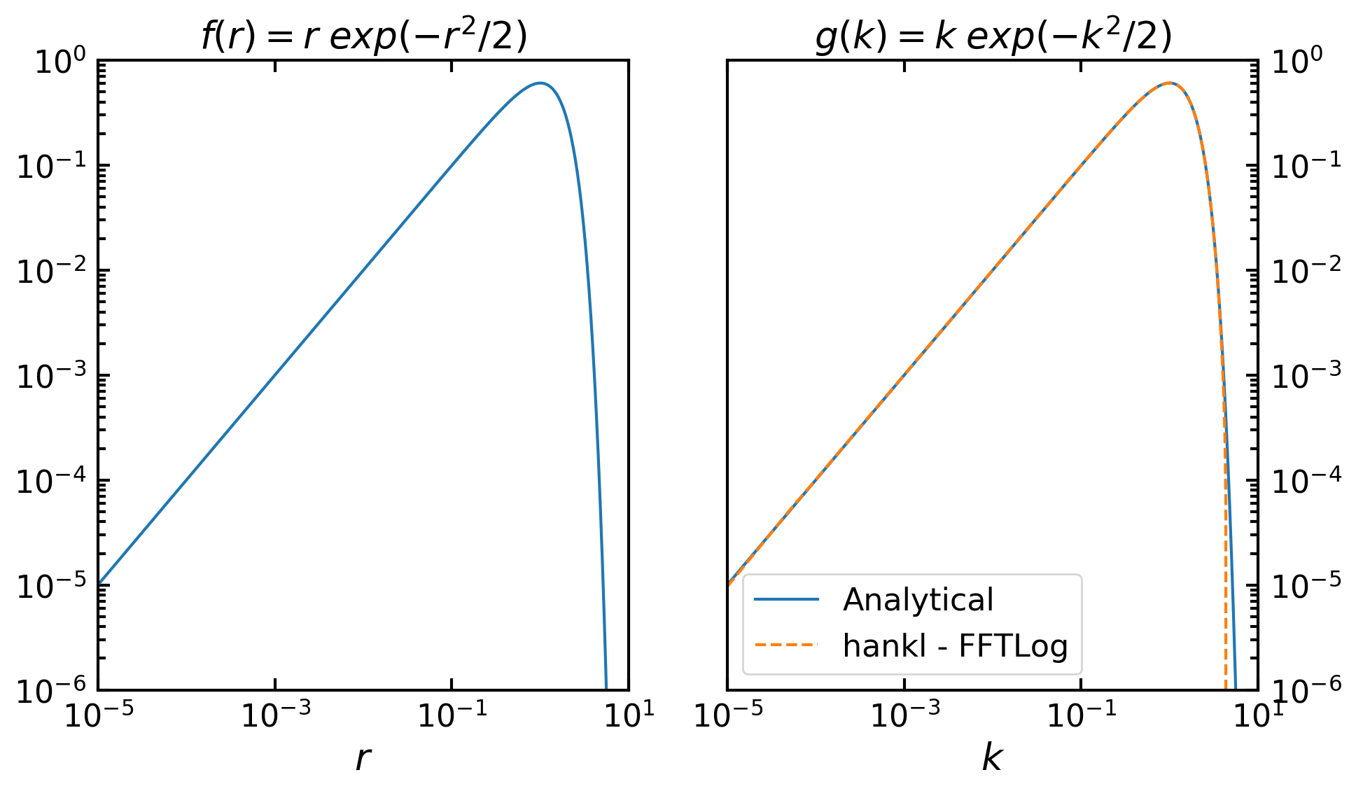
This is a simple example, used by Hamilton to illustrate how the FFTLog algorithm works. We will use hankl’s General FFTLog module to compute the following transform:

\[\int_{0}^{\infty} r^{\mu + 1} exp\Big(-\frac{r^{2}}{2}\Big) J_{\mu}(k r) k dr = k^{\mu+1} exp\Big(-\frac{k^{2}}{2}\Big)\]

Now in this example we know the analytical form of the result so we will use this to demonstrate the accuracy of the transformation.

The general form of the Hankel transform that hankl computes is the following:

\[g(k) = \int_0^\infty f(r) (kr)^{q} J_\mu(kr) k dr\]

This means that the function that we want to transform is:

\[f(r) = r^{\mu+1} exp\Big(-\frac{r^{2}}{2}\Big)\]

and the result should be

\[g(k) = k^{\mu+1} exp\Big(-\frac{k^{2}}{2}\Big)\]

which is of course the right hand side (RHS) of the first equation.

Now let’s start by importing everything we need:

import hankl
import numpy as np
import matplotlib.pyplot as pyplot

The next thing we want is to define the functions f(r) and g(r) as well as the integration range for r:

def f(r, mu=0.0):
    return r**(mu+1.0) * np.exp(-r**2.0 / 2.0)

def g(k, mu=0.0):
    return k**(mu+1.0) * np.exp(- k**2.0 / 2.0)

r = np.logspace(-5, 5, 2**10)

As you can see, we used an integration range for r which is quite wide and we also chose its size to be a power of two, this will make the algorithm faster and more accurate.

Now let’s perform the Hankel transform:

k, G = hankl.FFTLog(r, f(r, mu=0.0), q=0.0, mu=0.0)

Finally, we can plot the results:

plt.figure(figsize=(10,6))

ax1 = plt.subplot(121)
plt.loglog(r, f(r))
plt.title('$f(r) = r \; exp(-r^{2}/2)$')
plt.xlabel('$r$')
plt.ylim(10**(-6), 1)
plt.xlim(10**(-5), 10)

ax1.yaxis.tick_left()
ax2.yaxis.set_label_position("left")

ax2 = plt.subplot(122, sharey=ax1)
plt.loglog(k, g(k), label='Analytical')
plt.loglog(k, G, ls='--', label='hankl - FFTLog')
plt.title('$g(k) = k \; exp(-k^{2}/2)$')
plt.xlabel('$k$')
plt.ylim(10**(-6), 1)
plt.xlim(10**(-5), 10)
plt.legend()

ax2.yaxis.tick_right()
ax2.yaxis.set_label_position("right")
plt.tight_layout()

plt.show()

We can further impove the performace of hankl by enabling the ‘lowring’ option, extrapolating or zero/constant padding the function (See the API for more information).

Cosmology Example

In this example we will start from a model of the Galaxy Power Spectrum and our goal is to transform it to Configuration space to get the respective model for the Galaxy 2-Point Correlation Function. Furthermore, we want to transform both the Monopole and the Quadrupole of the Power Spectrum.

Let’s start by importing all the required packages; we will use classylss to get the Linear Matter Power Spectrum:

import hankl
import numpy as np
import matplotlib.pyplot as plt
import classylss
import classylss.binding as CLASS

Now that we have imported everything we need let’s initialize the fiducial Cosmology of our model:

engine = CLASS.ClassEngine({'H0':70, 'Omega_m':0.31})
bg = CLASS.Background(engine)
cosmo = CLASS.ClassEngine({'output': 'dTk vTk mPk', 'non linear': 'halofit', 'P_k_max_h/Mpc' : 20., "z_max_pk" : 100.0})
sp = CLASS.Spectra(cosmo)

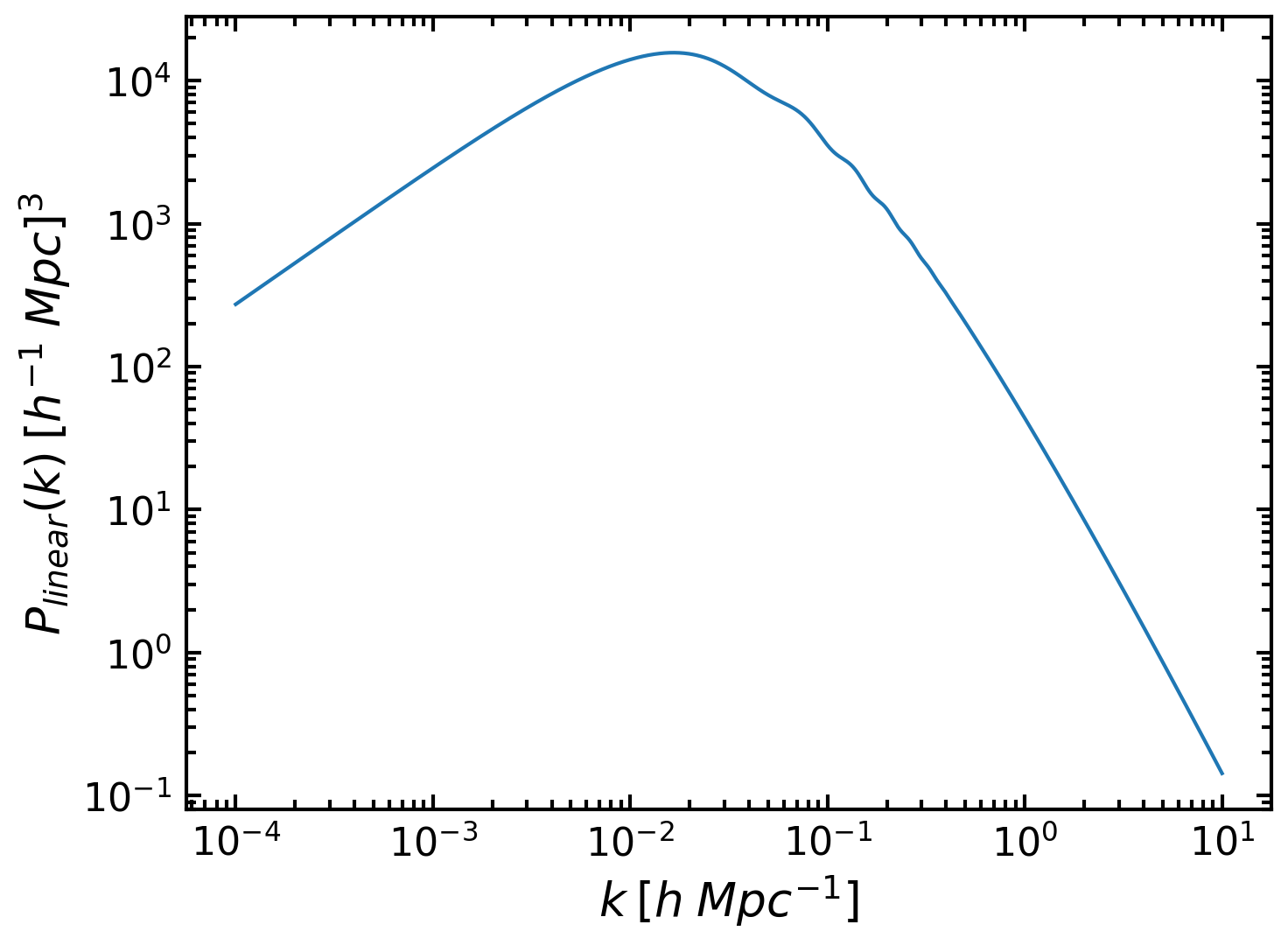
The next step is to define a suitable k range and get the model for the Linear Matter Power Spectrum:

k = np.logspace(-4, 1, 2**10)
pk_lin = sp.get_pklin(k=k, z=0.5)

where we also needed to specify the effective redshift z=0.5. We can plot easily the Linear Power Spectrum:

plt.loglog(k, pk_lin)
plt.xlabel(r'$k\: [h\; Mpc^{-1}]$')
plt.ylabel(r'$P_{linear}(k)\: [h^{-1}\; Mpc]^{3}$')
plt.show()

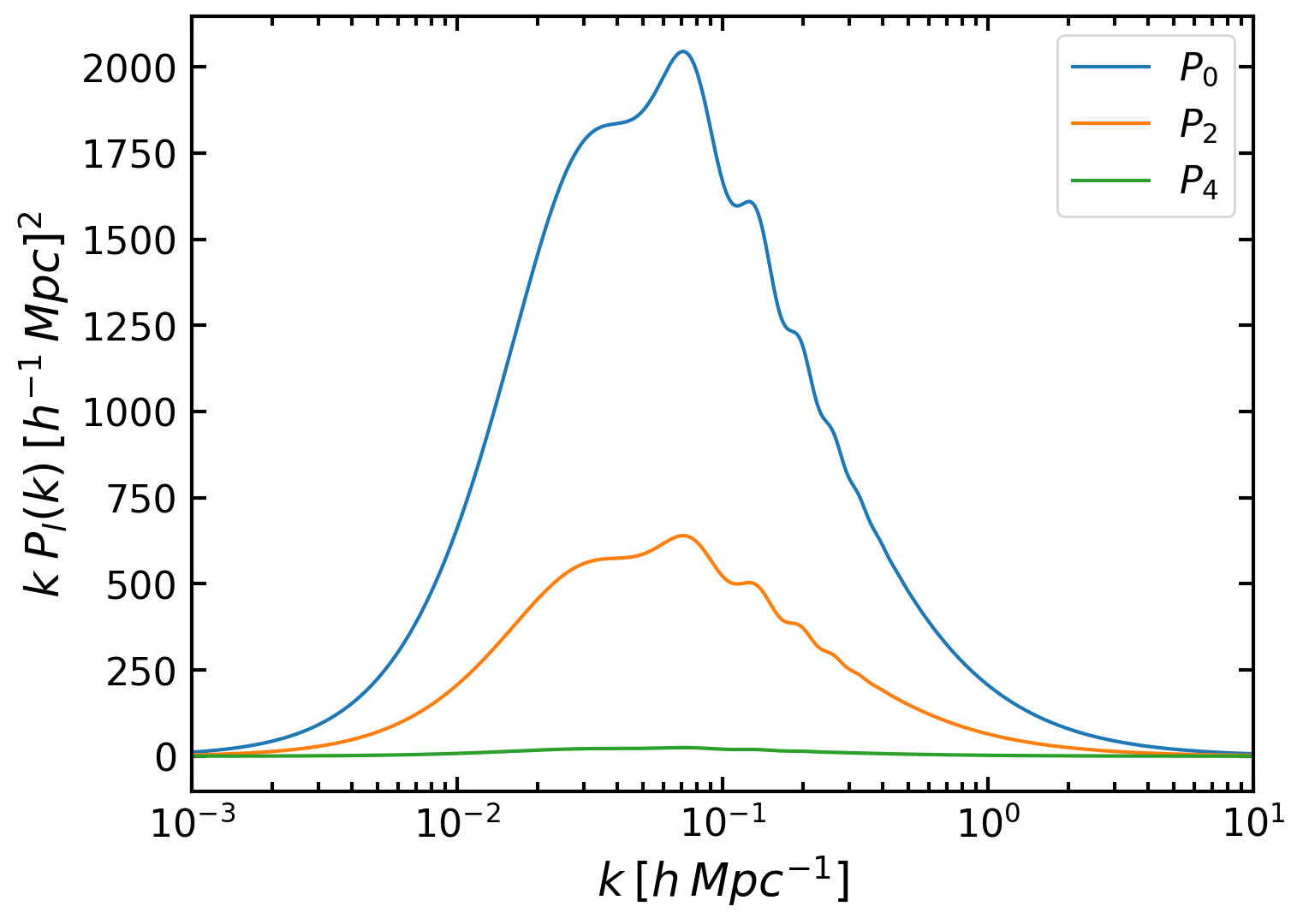
Now, this was the linear Matter Power Spectrum, to get the Galaxy Power Spectrum multipoles we will use Kaiser’s formula:

\[P(k, \mu) = (b + f \mu^{2})^{2} P_{lin}(k)\]

where \(b\) is the linear bias parameter, \(f\) is the logarithmic growth rate, and \(\mu\) is the cosine of the angle between teh Fourier modes and the line-of-sight. By decomposing the aforementioned function in terms of the Legendre polynomials we get the Monopole \((l=0)\), Quadrupole \((l=2)\) and Hexadecapole \((l=4)\) of the galaxy Power Spectrum:

def get_multipoles(b, f):

    p0 = (b*b + 2.0 * b *f / 3.0 + f*f/5.0 ) * pk_lin

    p2 = (4.0*b*f/3.0 + 4.0*f*f/7.0) * pk_lin

    p4 = (8.0* f*f / 35.0) * pk_lin

return p0, p2, p4

Alright, let’s compute and plot those multipoles for two realistic values of b and f:

P0, P2, P4 = get_multipoles(b=2.0, f=0.5)

plt.semilogx(k, k * P0, label=r'$P_{0}$')
plt.semilogx(k, k * P2, label=r'$P_{2}$')
plt.semilogx(k, k * P4, label=r'$P_{4}$')
plt.xlabel(r'$k \: [h\: Mpc^{-1}]$')
plt.ylabel(r'$k\; P_{l}(k) \: [h^{-1}\: Mpc]^{2}$')
plt.xlim(1e-3, 10)
plt.legend()
plt.show()

The last step involves using the Cosmology module P2xi to transform the above power spectrum multipoles to correlation function multipoles and plot them. Since the Hexadecapole (l=4) is almost zero, we will do the transform only for the Monopole and Quadrupole:

s, xi0 = hankl.P2xi(k, P0, l=0)
s, xi2 = hankl.P2xi(k, P2, l=2)

plt.plot(s, s*s*xi0, label=r'$s^{2}\xi_{0}$')
plt.plot(s, s*s*xi2, label=r'$s^{2}\xi_{2}$')
plt.xlim(20,180)
plt.ylim(-80,130)
plt.xlabel(r'$s\: (Mpc/h)$')
plt.ylabel(r'$s^{2} \xi_{l}$')
plt.legend()
plt.show()

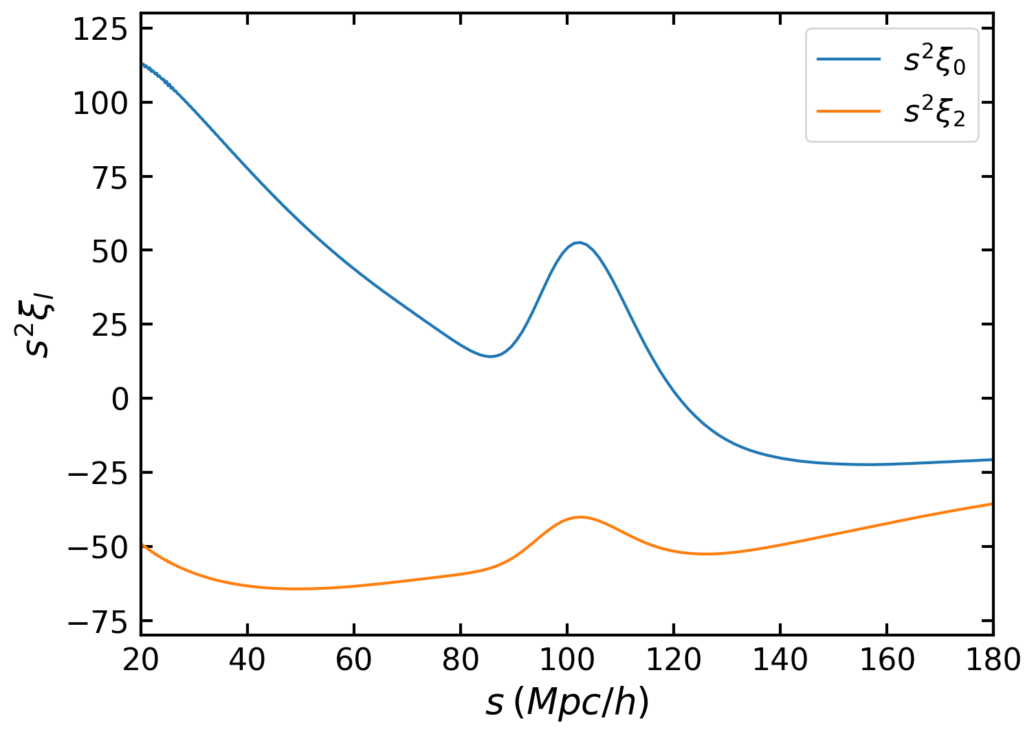
As expected we can see the Baryon Acoustic Oscillations (BAO) peak in both multipoles.